Nomogram
Intro
[This is a page from Jonathan Dushoff’s math wiki, adapted for use as a test of my Working Markup blog-post system. Scroll down for info about how this post is made, including source code. -lw]
On this page, I use the free software environment R to construct a nomogram that I read about in a recreational math book when I was a kid. This nomogram solves quadratic equations.
Nomogram
You can print out the nomogram, and use a ruler to read off the solutions to the quadratic equation, where the line from to intersects the scale.
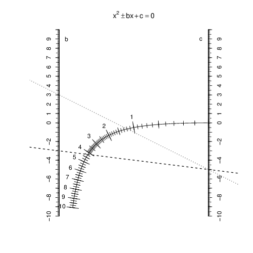
The example above shows the solutions to the equation . The dashed line connecting to shows the positive solution (4.2), and the dotted line connecting to shows the negative solution (-1.2).
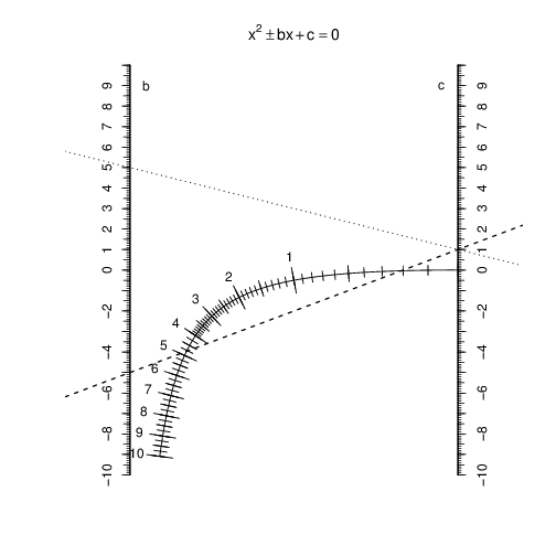
In this example (), both solutions are positive (0.2 and 4.8), thus only the dashed line intersects the scale.
Math
We want to draw lines from to that will pass through a point labeled with , where is a root, satisfying . The equation for our line is . Solve the quadratic to obtain , and substitute into the line equation to get .
If we want all lines corresponding to to go through our point, we must find one independent of . We do this by setting , to yield .
Code
Define and call a nomogram function.
Use make to make the example code below depend on the R environment from above (using our custom R rules).
Make a nomogram, then define and make example lines.
Here’s another example.
Printable
Export source code
This project is designed for reproducible research.
- This entire website (including the source text of this blog post, with all the source code included) is available for cloning at https://github.com/worden-lee/github-pages-sandbox. I’m planning to write instructions for processing it soon.
- To reproduce the full blog post you’ll need to have the following installed: Jekyll, git, R, latexml, GNU make, perl (and maybe other things - bug reports welcome).
- Here is an automatically-generated tar file of the source file contents: wmd_export.tgz. You should be able to unpack this directory and simply run ‘make example.Rout.png’ to build the first image above, and similar commands to build the other output files.
- To reproduce these outputs you will need GNU make, perl, and R installed.
To see the source text of this blog post, with the R and makefile code embedded, see https://github.com/worden-lee/github-pages-sandbox/blob/master/_posts/2014-10-15-nomogram.md.wmd.
See also a discussion of how this is put together at http://leeworden.net/lw/node/148 and http://leeworden.net/lw/node/149.