Sage Dynamics Demo

Intro

[This is an adaptation of a page from my open lab notebook wiki, as a demo of our Working Markup reproducible web-publishing system. Scroll down to the final section for info on how this post is made, including source code. -lw]

This post demonstrates a set of Sage classes I wrote to work with continuous-time dynamical systems, the kind of system my colleagues and I use a lot as mathematical models.

The computations in this blog post are implemented in two parts. The Sage class library is kept in a GitHub repository by itself, and the Sage scripts that use the library to implement a simple demo system on this page are stored as part of this page.

On this page I use those Sage classes to construct a simple population biology model of two populations, and analyze and evaluate it.

The Sage code for this model is below. Here’s its output, in LaTeX format:

The generic competition model:

	$\displaystyle\frac{dN_{1}}{dt}$	$\displaystyle=-\frac{{\left(N_{2}{\alpha_{12}}-K_{1}+N_{1}\right)}N_{1}r_{1}}{% K_{1}}$
	$\displaystyle\frac{dN_{2}}{dt}$	$\displaystyle=-\frac{{\left(N_{1}{\alpha_{21}}-K_{2}+N_{2}\right)}N_{2}r_{2}}{% K_{2}}$

The competition model with parameters bound to specific values:

	$\displaystyle\frac{dN_{1}}{dt}$	$\displaystyle=-\frac{1}{2}\,{\left(2\,N_{1}+N_{2}-2\right)}N_{1}$
	$\displaystyle\frac{dN_{2}}{dt}$	$\displaystyle=-\frac{1}{5}\,{\left(2\,N_{1}+4\,N_{2}-5\right)}N_{2}$

Equilibria of the generic model:

\left(\begin{array}[]{c}0\\ 0\end{array}\right),\left(\begin{array}[]{c}0\\ K_{2}\end{array}\right),\left(\begin{array}[]{c}K_{1}\\ 0\end{array}\right),\left(\begin{array}[]{c}\frac{K_{2}{\alpha_{12}}-K_{1}}{{% \alpha_{12}}{\alpha_{21}}-1}\\ \frac{K_{1}{\alpha_{21}}-K_{2}}{{\alpha_{12}}{\alpha_{21}}-1}\end{array}\right)

Stable equilibria of the bound model:

\left(\begin{array}[]{c}\frac{1}{2}\\ 1\end{array}\right)

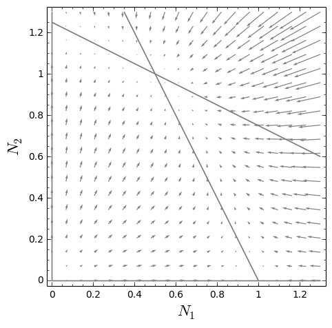
Here’s the state space plot that the program creates, showing a representative trajectory of the model’s dynamics, with flow vector field and zero-net-growth isoclines:

(ode-system-demo.png)

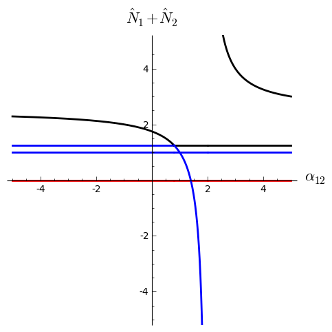
And a bifurcation diagram of total population vs. $\alpha_{12}$ (black=stable, red=repelling point, blue=saddle):

(bifurcation-diagram.png)

Source code

Here is the source code for this page’s demo:

ode-system-demo.sage.step

# produces: ode-system-demo.sage.out.tex ode-system-demo.png bifurcation-diagram.png

# use the dynamicalsystems module from SageDynamics
from dynamicalsystems import *

# I'll use a simple competition model borrowed from 
# http://www.tiem.utk.edu/~gross/bioed/bealsmodules/competition.html

# make variables for easy use
N_1, N_2, r_1, r_2, K_1, K_2 = SR.var( 'N_1, N_2, r_1, r_2, K_1, K_2' )
# alpha variables have special latex formatting for the double subscripts
alpha_12 = SR.var( 'alpha_12', latex_name='\\alpha_{12}' )
alpha_21 = SR.var( 'alpha_21', latex_name='\\alpha_{21}' )

# create the competition model by providing flow equations and state variables
comp_system_generic = ODESystem(
    { N_1: r_1 * N_1 * (K_1 - N_1 - alpha_12 * N_2) / K_1,
      N_2: r_2 * N_2 * (K_2 - alpha_21 * N_1 - N_2) / K_2 },
    [ N_1, N_2 ] )

# write output into a tex file
ltx = latex_output( 'ode-system-demo.sage.out.tex' )

ltx.write( 'The generic competition model:' )
ltx.write_block( comp_system_generic )

# and create a specific instantiation of the model by binding parameters
# it has a nontrivial solution if K_1/alpha_12 > K_2 and K_2/alpha_21 > K_1
comp_system_stable = comp_system_generic.bind( {
  K_1 : 1, K_2 : 5/4, alpha_12 : 1/2, alpha_21 : 1/2,
  r_1 : 1, r_2 : 1 } )

ltx.write( 'The competition model with parameters bound to specific values:' )
ltx.write_block( comp_system_stable )

# find the equilibria
ltx.write( 'Equilibria of the generic model: ' )
ltx.write( '\n\\[ ',
	', '.join( latex( column_vector( [ eq[hat(N_1)], eq[hat(N_2)] ] ) )
		for eq in comp_system_generic.equilibria() ),
	'\n\\]' )

# and check stability of the bound ones
ltx.write( 'Stable equilibria of the bound model: ' )
ltx.write( '\n\\[',
	', '.join( latex( column_vector( [ eq[hat(N_1)], eq[hat(N_2)] ] ) )
		for eq in comp_system_stable.stable_equilibria() ),
	'\n\\]' )

# solve numerically given starting time and initial conditions
s = comp_system_stable.solve( [0, 0.05, 0.02] )

# plot the system as a vector field on the x-y plane
p = comp_system_stable.plot_vector_field( (N_1,0,1.3), (N_2,0,1.3), color='gray', figsize=(5,5) )
# plot population nullclines
# (there is a plot_ZNGIs method for this, but to use it I'd need to
# be using the PopulationDynamicsSystem subclass)
p += comp_system_stable.plot_isoclines( (N_1,0,1.3), (N_2,0,1.3), [(N_1,0),(N_2,0)], color='gray' )
# superimpose the numerically-solved trajectory onto the same plot
p += s.plot( N_1, N_2, color='red' )
p.axes_labels( [ '$N_1$', '$N_2$' ] )
# render the plot into a png file
p.save( 'ode-system-demo.png' )

# and now do bifurcation diagram

# bind all parameters except the bifurcation parameter
comp_system_b = comp_system_generic.bind( {
  K_1 : 1, K_2 : 5/4, alpha_21 : 1/2, # bind everything except alpha_12
  r_1 : 1, r_2 : 1 } )
# and do plot of equilibrium population as a function of varying parameter
# alpha_12, color coded by whether the equilibrium is stable
comp_system_b.plot_bifurcation_diagram( (alpha_12, -5, 5), (hat(N_1) + hat(N_2), -5, 5), filename='bifurcation-diagram.png', figsize=(5,5) )

# and close the latex output
ltx.close()

And a small makefile to get the above Sage code to connect with the libraries pulled from GitHub into a separate directory:

Reproducibility

Here are instructions to run this Sage code yourself. You will need Sage, GNU make, git, perl, and maybe some other utilities installed.

Download and unpack the source code from this page: wmd_export.tgz
Install Sage and the Sage library code from https://github.com/worden-lee/SageDynamics
In the code directory, run make ode-system-demo.sage.out.tex

To see how this blog post is written, with source code embedded, see https://github.com/worden-lee/github-pages-sandbox/blob/master/_posts/2014-10-20-SageDynamics.markdown.wmd.